
原文链接:https://blog.csdn.net/x454045816/article/details/108744637
一、算法介绍
蚁群算法,最早是1992年由Marco Dorigo在他的博士论文中提出的,是一种通过模拟自然界蚂蚁寻径的行为,提出的一种全新的模拟进化算法。据昆虫学家的观察和研究发现,生物世界中的蚂蚁有能力在没有任何可见提示下找到从其巢穴到食物源的最短路径,并能随环境的变化而变化,适应性地搜索新的路径,产生新的选择。这是因为蚂蚁在寻找路径时会在路径上释放一种特殊的分泌物——信息素,使得一定范围内的其他蚂蚁能够觉察并影响它们以后的寻径行为。当一些路径上通过的蚂蚁越来越多时,该路径上的信息素浓度就越大,后来的蚂蚁选择该路径的可能性就越大,从而进一步增加了该路径上的信息素浓度,这种选择过程称为蚂蚁的自催化行为
二、基本思想
- 根据具体问题设置多只蚂蚁,分头并行搜索。
- 每只蚂蚁完成一次周游后,在行进的路上释放信息素,信息素量与解的质量成正比。
- 蚂蚁路径的选择根据信息素强度大小(初始信息素量设为相等),同时考虑两点之间的距离,采用随机的局部搜索策略。这使得距离较短的边,其上的信息素量较大,后来的蚂蚁选择该边的概率也较大。
- 每只蚂蚁只能走合法路线(经过每个城市1次且仅1次),为此设置禁忌表来控制。
- 所有蚂蚁都搜索完一次就是迭代一次,每迭代一次就对所有的边做一次信息素更新,原来的蚂蚁死掉,新的蚂蚁进行新一轮搜索。
- 更新信息素包括原有信息素的蒸发和经过的路径上信息素的增加。
- 达到预定的迭代步数,或出现停滞现象(所有蚂蚁都选择同样的路径,解不再变化),则算法结束,以当前最优解作为问题的最优解。
三、算法流程
1. 初始化参数:开始时,每条边的信息素量都相等</p>
2. 将各只蚂蚁放置各顶点,禁忌表为对应的顶点。</p>
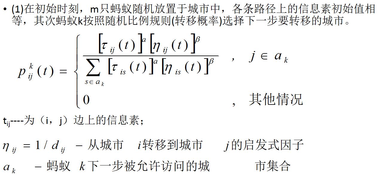
3. 取1只蚂蚁,计算转移概率 ,按照轮 盘赌的方式选择下一个顶点,更新禁忌表,再计算概率,再选择顶点,再更新禁忌表,直至遍历所有顶点一次。</p>
4.计算该只蚂蚁留在各边的信息素量 ,该蚂蚁死去。</p>
5. 重复3-4步,直至m只蚂蚁都周游完毕。</p>
6. 计算各边的信息素增量 和信息素量 。</p>
7. 计算本次迭代的路径,更新当前的最优路径,清空禁忌表。</p>
8. 判断是否达到预定的迭代步数,或者是否出现停滞现象,若是则算法结束,输出当前最优路径,否则转到步骤2,进行下一次迭代。
第一个是转移城市概率公式:
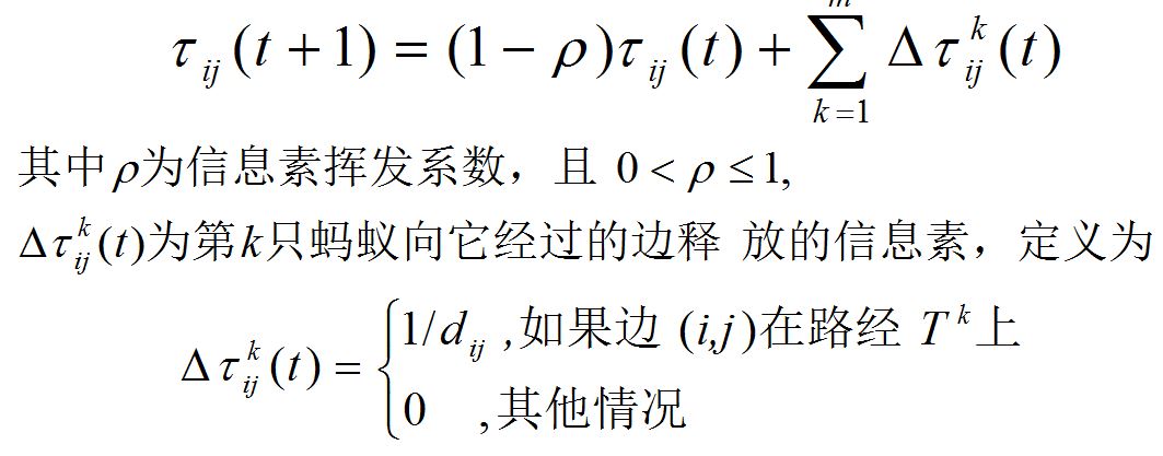
第二个公式是:信息素更新公式
aco
# -*- coding: utf-8 -*-
"""
Created on Wed Jun 16 15:21:03 2018
@author: SYSTEM
"""
import os

os.getcwd()
#返回当前工作目录
import numpy as np
import matplotlib.pyplot as plt
import math
# % pylab
#初始化城市坐标,总共52个城市
coordinates = np.array([[565.0, 575.0], [25.0, 185.0], [345.0, 750.0], [945.0, 685.0], [845.0, 655.0],
                        [880.0, 660.0], [25.0, 230.0], [525.0, 1000.0], [580.0, 1175.0], [650.0, 1130.0],
                        [1605.0, 620.0], [1220.0, 580.0], [1465.0, 200.0], [1530.0, 5.0], [845.0, 680.0],
                        [725.0, 370.0], [145.0, 665.0], [415.0, 635.0], [510.0, 875.0], [560.0, 365.0],
                        [300.0, 465.0], [520.0, 585.0], [480.0, 415.0], [835.0, 625.0], [975.0, 580.0],
                        [1215.0, 245.0], [1320.0, 315.0], [1250.0, 400.0], [660.0, 180.0], [410.0, 250.0],
                        [420.0, 555.0], [575.0, 665.0], [1150.0, 1160.0], [700.0, 580.0], [685.0, 595.0],
                        [685.0, 610.0], [770.0, 610.0], [795.0, 645.0], [720.0, 635.0], [760.0, 650.0],
                        [475.0, 960.0], [95.0, 260.0], [875.0, 920.0], [700.0, 500.0], [555.0, 815.0],
                        [830.0, 485.0], [1170.0, 65.0], [830.0, 610.0], [605.0, 625.0], [595.0, 360.0],
                        [1340.0, 725.0], [1740.0, 245.0]])

#计算52个城市间的欧式距离
def getdistmat(coordinates):
    num = coordinates.shape[0]
    distmat = np.zeros((52, 52))
    # 初始化生成52*52的矩阵
    for i in range(len(coordinates)):
        xi,yi = coordinates[i][0],coordinates[i][1]
        for j in range(len(coordinates)):
            xj,yj = coordinates[j][0],coordinates[j][1]
            if (xi==xj) & (yi==yj):
                distmat[i,j] = round(0)
            else:
                #distmat[i,j] = round(math.sqrt((xi-xj)**2+(yi-yj)**2),2)
                distmat[i,j] = round(math.sqrt((xi-xj)**2+(yi-yj)**2))
    return distmat
#返回城市距离矩阵


distmat = getdistmat(coordinates)
print distmat

numant = 60  # 蚂蚁个数
numcity = coordinates.shape[0]
# shape[0]=52 城市个数,也就是任务个数
alpha = 1  # 信息素重要程度因子
beta = 3   # 启发函数重要程度因子
rho = 0.1  # 信息素的挥发速度
Q = 1      # 完成率

iter = 0       #迭代初始
itermax = 500  #迭代总数
#print np.diag([1e10] * numcity)
etatable = 1.0 / (distmat + np.diag([1e10] * numcity))
#print etatable
#diag(),将一维数组转化为方阵 启发函数矩阵,表示蚂蚁从城市i转移到城市j的期望程度
pheromonetable = np.ones((numcity, numcity))
# 信息素矩阵 52*52
pathtable = np.zeros((numant, numcity)).astype(int)
# 路径记录表,转化成整型 40*52
distmat = getdistmat(coordinates)
# 城市的距离矩阵 52*52

lengthaver = np.zeros(itermax)  # 迭代50次,存放每次迭代后,路径的平均长度  50*1
lengthbest = np.zeros(itermax)  # 迭代50次,存放每次迭代后,最佳路径长度  50*1
pathbest = np.zeros((itermax, numcity))  # 迭代50次,存放每次迭代后,最佳路径城市的坐标 50*52

while iter < itermax:
    #迭代总数

    #40个蚂蚁随机放置于52个城市中
    if numant <= numcity:  # 城市数比蚂蚁数多,不用管
        pathtable[:, 0] = np.random.permutation(range(1,numcity))[:numant-1]
        #返回一个打乱的40*52矩阵,但是并不改变原来的数组,把这个数组的第一列(40个元素)放到路径表的第一列中
        #矩阵的意思是哪个蚂蚁在哪个城市,矩阵元素不大于52
    else:  # 蚂蚁数比城市数多,需要有城市放多个蚂蚁
        pathtable[:numcity, 0] = np.random.permutation(range(numcity))[:]
        # 先放52个
        pathtable[numcity:, 0] = np.random.permutation(range(numcity))[:numant - numcity]
        # 再把剩下的放完
        # print(pathtable[:,0])
    #print pathtable
    length = np.zeros(numant)  # 1*40的数组

    #本段程序算出每只/第i只蚂蚁转移到下一个城市的概率
    for i in range(numant):

        # i=0
        visiting = pathtable[i, 0]  # 当前所在的城市
        # set()创建一个无序不重复元素集合
        # visited = set() #已访问过的城市,防止重复
        # visited.add(visiting) #增加元素
        unvisited = set(range(numcity))
        #未访问的城市集合
        #剔除重复的元素
        unvisited.remove(visiting)  # 删除已经访问过的城市元素

        for j in range(1, numcity):  # 循环numcity-1次,访问剩余的所有numcity-1个城市
            # j=1
            # 每次用轮*盘法选择下一个要访问的城市
            listunvisited = list(unvisited)
            #未访问城市数,list
            probtrans = np.zeros(len(listunvisited))
            #每次循环都初始化转移概率矩阵1*52,1*51,1*50,1*49....


            #以下是计算转移概率
            for k in range(len(listunvisited)):
                probtrans[k] = np.power(pheromonetable[visiting][listunvisited[k]], alpha) \
                               * np.power(etatable[visiting][listunvisited[k]], beta)
            #eta-从城市i到城市j的启发因子 这是概率公式的分母   其中[visiting][listunvis[k]]是从本城市到k城市的信息素
            cumsumprobtrans = (probtrans / sum(probtrans)).cumsum()
            #求出本只蚂蚁的转移到各个城市的概率斐波衲挈数列

            cumsumprobtrans -= np.random.rand()
            # 随机生成下个城市的转移概率,再用区间比较
            # k = listunvisited[find(cumsumprobtrans > 0)[0]]
            k = listunvisited[list(cumsumprobtrans > 0).index(True)]
            # k = listunvisited[np.where(cumsumprobtrans > 0)[0]]
            # where 函数选出符合cumsumprobtans>0的数
            # 下一个要访问的城市

            pathtable[i, j] = k
            #采用禁忌表来记录蚂蚁i当前走过的第j城市的坐标,这里走了第j个城市.k是中间值
            unvisited.remove(k)
            # visited.add(k)
            #将未访问城市列表中的K城市删去,增加到已访问城市列表中

            length[i] += distmat[visiting][k]
            #计算本城市到K城市的距离
            visiting = k

        length[i] += distmat[visiting][pathtable[i, 0]]
        # 计算本只蚂蚁的总的路径距离,包括最后一个城市和第一个城市的距离

    # print("ants all length:",length)
    # 包含所有蚂蚁的一个迭代结束后,统计本次迭代的若干统计参数

    lengthaver[iter] = length.mean()
    #本轮的平均路径


    #本部分是为了求出最佳路径

    if iter == 0:
        lengthbest[iter] = length.min()
        pathbest[iter] = pathtable[length.argmin()].copy()
    #如果是第一轮路径,则选择本轮最短的路径,并返回索引值下标,并将其记录
    else:
    #后面几轮的情况,更新最佳路径
        if length.min() > lengthbest[iter - 1]:
            lengthbest[iter] = lengthbest[iter - 1]
            pathbest[iter] = pathbest[iter - 1].copy()
        # 如果是第一轮路径,则选择本轮最短的路径,并返回索引值下标,并将其记录
        else:
            lengthbest[iter] = length.min()
            pathbest[iter] = pathtable[length.argmin()].copy()


    #此部分是为了更新信息素
    changepheromonetable = np.zeros((numcity, numcity))
    for i in range(numant):#更新所有的蚂蚁
        for j in range(numcity - 1):
            changepheromonetable[pathtable[i, j]][pathtable[i, j + 1]] += Q / distmat[pathtable[i, j]][pathtable[i, j + 1]]
            #根据公式更新本只蚂蚁改变的城市间的信息素      Q/d   其中d是从第j个城市到第j+1个城市的距离
        changepheromonetable[pathtable[i, j + 1]][pathtable[i, 0]] += Q / distmat[pathtable[i, j + 1]][pathtable[i, 0]]
        #首城市到最后一个城市 所有蚂蚁改变的信息素总和

    #信息素更新公式p=(1-挥发速率)*现有信息素+改变的信息素
    pheromonetable = (1 - rho) * pheromonetable + changepheromonetable

    iter += 1  # 迭代次数指示器+1
    print("this iteration end:",iter)
    # 观察程序执行进度,该功能是非必须的
    if (iter - 1) % 20 == 0:
        print("schedule:",iter - 1)
#迭代完成


#以下是做图部分
#做出平均路径长度和最优路径长度
fig, axes = plt.subplots(nrows=2, ncols=1, figsize=(12, 10))
axes[0].plot(lengthaver, 'k', marker='*')
axes[0].set_title('Average Length')
axes[0].set_xlabel(u'iteration')

#线条颜色black https://blog.csdn.net/ywjun0919/article/details/8692018
#axes[1].plot(lengthbest, 'k', marker='<')
axes[1].set_title('Best Length')
axes[1].set_xlabel(u'iteration')
#fig.savefig('Average_Best.png', dpi=500, bbox_inches='tight')
#plt.close()
#fig.show()

# 作出找到的最优路径图
bestpath = pathbest[-1]

plt.plot(coordinates[:, 0], coordinates[:, 1], 'r.', marker='>')
plt.xlim([-100, 2000])
#x范围
plt.ylim([-100, 1500])
#y范围

for i in range(numcity - 1):
    #按坐标绘出最佳两两城市间路径
    m, n = int(bestpath[i]), int(bestpath[i + 1])
    print("best_path:",m, n)
    plt.plot([coordinates[m][0],coordinates[n][0]],   [coordinates[m][1], coordinates[n][1]],  'k')

plt.plot([coordinates[int(bestpath[0])][0],coordinates[int(bestpath[51])][0]],    [coordinates[int(bestpath[0])][1],coordinates[int(bestpath[51])][1]]   ,'b')
print lengthbest.min()
#ax = plt.gca()
#ax.set_title("Best Path")
#ax.set_xlabel('X_axis')
#ax.set_ylabel('Y_axis')

#plt.savefig('Best Path.png', dpi=500, bbox_inches='tight')
#plt.close()
pso
import math
import random
import pandas as pd
import matplotlib.pyplot as plt
from matplotlib.pylab import mpl
import numpy as np


#计算52个城市间的欧式距离
def getdistmat(coordinates):
    num = coordinates.shape[0]
    distmat = np.zeros((num, num))
    # 初始化生成52*52的矩阵
    for i in range(len(coordinates)):
        xi,yi = coordinates[i][0],coordinates[i][1]
        for j in range(len(coordinates)):
            xj,yj = coordinates[j][0],coordinates[j][1]
            if (xi==xj) & (yi==yj):
                distmat[i,j] = round(0)
            else:
                distmat[i,j] = int(math.sqrt((xi-xj)**2+(yi-yj)**2))
    return distmat
#返回城市距离矩阵


def calFitness(line,dis_matrix):
    '''
    计算路径距离,即评价函数
    输入:line-路径,dis_matrix-城市间距离矩阵;
    输出:路径距离-dis_sum
    '''
    dis_sum = 0
    dis = 0
    for i in range(len(line)-1):
        dis = dis_matrix[line[i],line[i+1]]#计算距离
        dis_sum = dis_sum+dis
    dis = dis_matrix[line[-1],line[0]]
    dis_sum = dis_sum+dis
    return round(dis_sum,1)


def draw_path(line,CityCoordinates):
    '''
    #画路径图
    输入:line-路径,CityCoordinates-城市坐标;
    输出:路径图
    '''
    x,y= [],[]
    for i in line:
        Coordinate = CityCoordinates[i]
        x.append(Coordinate[0])
        y.append(Coordinate[1])
    x.append(x[0])
    y.append(y[0])
    plt.plot(x, y,'r-', color='#4169E1', alpha=0.8, linewidth=0.8)
    plt.xlabel('x')
    plt.ylabel('y')
    plt.show()


def crossover(bird,pLine,gLine,w,c1,c2):
    croBird = [None]*len(bird)#初始化
    parent1 = bird#选择parent1
    #选择parent2(轮*盘赌操作)
    randNum = random.uniform(0, sum([w,c1,c2]))
    if randNum <= w:
        parent2 = [bird[i] for i in range(len(bird)-1,-1,-1)]#bird的逆序
    elif randNum <= w+c1:
        parent2 = pLine
    else:
        parent2 = gLine

    #parent1-> croBird
    start_pos = random.randint(0,len(parent1)-1)
    end_pos = random.randint(0,len(parent1)-1)
    if start_pos>end_pos:start_pos,end_pos = end_pos,start_pos
    croBird[start_pos:end_pos+1] = np.copy(parent1[start_pos:end_pos+1])

    # parent2 -> croBird
    list1 = list(range(0,start_pos))
    list2 = list(range(end_pos+1,len(parent2)))
    list_index = list1+list2#croBird从后往前填充
    j = -1
    for i in list_index:
        for j in range(j+1,len(parent2)+1):
            if parent2[j] not in croBird:
                croBird[i] = parent2[j]
                break

    return croBird


#参数
CityNum = 52#城市数量
MinCoordinate = 0#二维坐标最小值
MaxCoordinate = 101#二维坐标最大值
iterMax = 1000#迭代次数
iterI = 1#当前迭代次数

#PSO参数
birdNum = 100#粒子数量
w = 0.3#惯性因子
c1 = 0.3#自我认知因子
c2 = 0.4#社会认知因子
pBest,pLine =0,[]#当前最优值、当前最优解,(自我认知部分)
gBest,gLine = 0,[]#全局最优值、全局最优解,(社会认知部分)

#初始化城市坐标,总共52个城市
coordinates = np.array([[565.0, 575.0], [25.0, 185.0], [345.0, 750.0], [945.0, 685.0], [845.0, 655.0],
                        [880.0, 660.0], [25.0, 230.0], [525.0, 1000.0], [580.0, 1175.0], [650.0, 1130.0],
                        [1605.0, 620.0], [1220.0, 580.0], [1465.0, 200.0], [1530.0, 5.0], [845.0, 680.0],
                        [725.0, 370.0], [145.0, 665.0], [415.0, 635.0], [510.0, 875.0], [560.0, 365.0],
                        [300.0, 465.0], [520.0, 585.0], [480.0, 415.0], [835.0, 625.0], [975.0, 580.0],
                        [1215.0, 245.0], [1320.0, 315.0], [1250.0, 400.0], [660.0, 180.0], [410.0, 250.0],
                        [420.0, 555.0], [575.0, 665.0], [1150.0, 1160.0], [700.0, 580.0], [685.0, 595.0],
                        [685.0, 610.0], [770.0, 610.0], [795.0, 645.0], [720.0, 635.0], [760.0, 650.0],
                        [475.0, 960.0], [95.0, 260.0], [875.0, 920.0], [700.0, 500.0], [555.0, 815.0],
                        [830.0, 485.0], [1170.0, 65.0], [830.0, 610.0], [605.0, 625.0], [595.0, 360.0],
                        [1340.0, 725.0], [1740.0, 245.0]])
dis_matrix = getdistmat(coordinates)#计算城市间距离,生成矩阵

birdPop = [random.sample(range(len(coordinates)),len(coordinates)) for i in range(birdNum)]#初始化种群,随机生成
fits = [calFitness(birdPop[i],dis_matrix) for i in range(birdNum)]#计算种群适应度
gBest = pBest = min(fits)#全局最优值、当前最优值
gLine = pLine = birdPop[fits.index(min(fits))]#全局最优解、当前最优解

while iterI <= iterMax:#迭代开始
    for i in range(len(birdPop)):
        birdPop[i] = crossover(birdPop[i],pLine,gLine,w,c1,c2)
        fits[i] = calFitness(birdPop[i],dis_matrix)

    pBest,pLine =  min(fits),birdPop[fits.index(min(fits))]
    if min(fits) <= gBest:
        gBest,gLine =  min(fits),birdPop[fits.index(min(fits))]

    if (iterI % 20 == 0):
      print(iterI,gBest)#打印当前代数和最佳适应度值
    iterI += 1#迭代计数加一

print(gLine)#路径顺序
print(gBest)
draw_path(gLine,coordinates)#画路径图
alns
# Adaptive Large Neighborhood Search
import numpy as np
import random as rd
import copy
import matplotlib.pyplot as plt
import math

destory_num = 7
#初始化城市坐标,总共52个城市
coordinates = np.array([[565.0, 575.0], [25.0, 185.0], [345.0, 750.0], [945.0, 685.0], [845.0, 655.0],
                        [880.0, 660.0], [25.0, 230.0], [525.0, 1000.0], [580.0, 1175.0], [650.0, 1130.0],
                        [1605.0, 620.0], [1220.0, 580.0], [1465.0, 200.0], [1530.0, 5.0], [845.0, 680.0],
                        [725.0, 370.0], [145.0, 665.0], [415.0, 635.0], [510.0, 875.0], [560.0, 365.0],
                        [300.0, 465.0], [520.0, 585.0], [480.0, 415.0], [835.0, 625.0], [975.0, 580.0],
                        [1215.0, 245.0], [1320.0, 315.0], [1250.0, 400.0], [660.0, 180.0], [410.0, 250.0],
                        [420.0, 555.0], [575.0, 665.0], [1150.0, 1160.0], [700.0, 580.0], [685.0, 595.0],
                        [685.0, 610.0], [770.0, 610.0], [795.0, 645.0], [720.0, 635.0], [760.0, 650.0],
                        [475.0, 960.0], [95.0, 260.0], [875.0, 920.0], [700.0, 500.0], [555.0, 815.0],
                        [830.0, 485.0], [1170.0, 65.0], [830.0, 610.0], [605.0, 625.0], [595.0, 360.0],
                        [1340.0, 725.0], [1740.0, 245.0]])

#计算52个城市间的欧式距离
def getdistmat(coordinates):
    num = coordinates.shape[0]
    distmat = np.zeros((num, num))
    # 初始化生成52*52的矩阵
    for i in range(len(coordinates)):
        xi,yi = coordinates[i][0],coordinates[i][1]
        for j in range(len(coordinates)):
            xj,yj = coordinates[j][0],coordinates[j][1]
            if (xi==xj) & (yi==yj):
                distmat[i,j] = round(0)
            else:
                distmat[i,j] = int(math.sqrt((xi-xj)**2+(yi-yj)**2))
    return distmat
#返回城市距离矩阵


distmat = getdistmat(coordinates)
print distmat
numcity = coordinates.shape[0]

'''
distmat = np.array([[0,350,290,670,600,500,660,440,720,410,480,970],
                 [350,0,340,360,280,375,555,490,785,760,700,1100],
                 [290,340,0,580,410,630,795,680,1030,695,780,1300],
                 [670,360,580,0,260,380,610,805,870,1100,1000,1100],
                 [600,280,410,260,0,610,780,735,1030,1000,960,1300],
                 [500,375,630,380,610,0,160,645,500,950,815,950],
                 [660,555,795,610,780,160,0,495,345,820,680,830],
                 [440,490,680,805,735,645,495,0,350,435,300,625],
                 [720,785,1030,870,1030,500,345,350,0,475,320,485],
                 [410,760,695,1100,1000,950,820,435,475,0,265,745],
                 [480,700,780,1000,960,815,680,300,320,265,0,585],
                 [970,1100,1300,1100,1300,950,830,625,485,745,585,0]])
'''

def disCal(path):             # calculate distance
    distance = 0
    for i in range(0, len(path) - 1):
        distance += distmat[path[i]][path[i + 1]]
    distance += distmat[path[-1]][path[0]]
    return distance

def selectAndUseDestroyOperator(destroyWeight,currentSolution):    # select and use destroy operators
    destroyOperator = -1
    sol = copy.deepcopy(currentSolution)
    destroyRoulette = np.array(destroyWeight).cumsum()
    r = rd.uniform(0, max(destroyRoulette))
    for i in range(len(destroyRoulette)):
        if destroyRoulette[i] >= r:
            if i == 0:
                destroyOperator = i
                removedCities = randomDestroy(sol)
                destroyUseTimes[i] += 1
                break
            elif i == 1:
                destroyOperator = i
                removedCities = max3Destroy(sol)
                destroyUseTimes[i] += 1
                break
    return sol,removedCities,destroyOperator

def selectAndUseRepairOperator(repairWeight,destroyedSolution,removeList):    # select and use repair operators
    repairOperator = -1
    repairRoulette = np.array(repairWeight).cumsum()
    r = rd.uniform(0, max(repairRoulette))
    i=1
    #for i in range(len(repairRoulette)):
    #    if repairRoulette[i] >= r:
    if i == 0:
        repairOperator = i
        randomInsert(destroyedSolution,removeList)
        repairUseTimes[i] += 1
    #    break
    elif i == 1:
        repairOperator = i
        greedyInsert(destroyedSolution,removeList)
        repairUseTimes[i] += 1
    #    break
    return destroyedSolution,repairOperator

def randomDestroy(sol):    # randomly remove 3 cities
    solNew = copy.deepcopy(sol)
    removed = []
    removeIndex = rd.sample(range(0, distmat.shape[0]), destory_num)
    for i in removeIndex:
        removed.append(solNew[i])
        sol.remove(solNew[i])
    return removed

def max3Destroy(sol):      # remove city with 3 longest segments
    solNew = copy.deepcopy(sol)
    removed = []
    dis = []
    for i in range(len(sol) - 1):
        dis.append(distmat[sol[i]][sol[i + 1]])
    dis.append(distmat[sol[-1]][sol[0]])
    disSort = copy.deepcopy(dis)
    disSort.sort()
    for i in range(destory_num):
        if dis.index(disSort[len(disSort) - i - 1]) == len(dis) - 1:
            removed.append(solNew[0])
            sol.remove(solNew[0])
        else:
            removed.append(solNew[dis.index(disSort[len(disSort) - i - 1]) + 1])
            sol.remove(solNew[dis.index(disSort[len(disSort) - i - 1]) + 1])
    return removed

def randomInsert(sol,removeList):     # randomly insert 3 cities
    insertIndex = rd.sample(range(0, distmat.shape[0]), destory_num)
    for i in range(len(insertIndex)):
        sol.insert(insertIndex[i],removeList[i])

def greedyInsert(sol,removeList):     # greedy insertion
    dis = float("inf")
    insertIndex = -1
    for i in range(len(removeList)):
        for j in range(len(sol) + 1):
            solNew = copy.deepcopy(sol)
            solNew.insert(j,removeList[i])
            if disCal(solNew) < dis:
                dis = disCal(solNew)
                insertIndex = j
        sol.insert(insertIndex,removeList[i])
        dis = float("inf")

T = 200
a = 0.9
b = 0.5
wDestroy = [1 for i in range(2)]     # weights of the destroy operators
wRepair = [1 for i in range(2)]      # weights of the repair operators
destroyUseTimes = [0 for i in range(2)]     #The number of times the destroy operator has been used
repairUseTimes = [0 for i in range(2)]      #The number of times the repair operator has been used
destroyScore = [1 for i in range(2)]      # the score of destroy operators
repairScore = [1 for i in range(2)]       # the score of repair operators
solution = [i for i in range(distmat.shape[0])] # initial solution
bestSolution = copy.deepcopy(solution)  # best solution
iterx, iterxMax = 0, 20

if __name__ == '__main__':
    lengthaver = []
    lengthbest = []
    while iterx < iterxMax:       # while stop criteria not met
        while T > 10:
            destroyedSolution,remove,destroyOperatorIndex = selectAndUseDestroyOperator(wDestroy,solution)
            newSolution,repairOperatorIndex = selectAndUseRepairOperator(wRepair,destroyedSolution,remove)

            if disCal(newSolution) <= disCal(solution):
                solution = newSolution
                if disCal(newSolution) <= disCal(bestSolution):
                    bestSolution = newSolution

                    destroyScore[destroyOperatorIndex] += 1.4     # update the score of the operators
                    repairScore[repairOperatorIndex] += 1.4
                else:
                    destroyScore[destroyOperatorIndex] += 1.1
                    repairScore[repairOperatorIndex] += 1.1
            else:
                if rd.random() < np.exp(- disCal(newSolution)/ T):  # the simulated annealing acceptance criteria
                    solution = newSolution
                    destroyScore[destroyOperatorIndex] += 0.9
                    repairScore[repairOperatorIndex] += 0.9
                else:
                    destroyScore[destroyOperatorIndex] += 0.6
                    repairScore[repairOperatorIndex] += 0.6

            wDestroy[destroyOperatorIndex] = wDestroy[destroyOperatorIndex] * b + (1 - b) * \
                                             (destroyScore[destroyOperatorIndex] / destroyUseTimes[destroyOperatorIndex])
            wRepair[repairOperatorIndex] = wRepair[repairOperatorIndex] * b + (1 - b) * \
                                           (repairScore[repairOperatorIndex] / repairUseTimes[repairOperatorIndex])
            # update the weight of the operators
            T = a * T
            lengthaver.append(disCal(solution))
        iterx += 1
        T = 100


    lengthbest = lengthaver
    #以下是做图部分
    #做出平均路径长度和最优路径长度
    fig, axes = plt.subplots(nrows=2, ncols=1, figsize=(12, 10))
    axes[0].plot(lengthaver, 'k', marker='*')
    axes[0].set_title('Average Length')
    axes[0].set_xlabel(u'iteration')

    #线条颜色black https://blog.csdn.net/ywjun0919/article/details/8692018
    axes[1].plot(lengthaver, 'k', marker='<')
    axes[1].set_title('Best Length')
    axes[1].set_xlabel(u'iteration')

    # 作出找到的最优路径图
    bestpath = bestSolution

    plt.plot(coordinates[:, 0], coordinates[:, 1], 'r.', marker='>')
    plt.xlim([-100, 2000])
    #x范围
    plt.ylim([-100, 1500])
    #y范围

    for i in range(numcity - 1):
        #按坐标绘出最佳两两城市间路径
        m, n = int(bestpath[i]), int(bestpath[i + 1])
        print("best_path:",m, n)
        plt.plot([coordinates[m][0],coordinates[n][0]],   [coordinates[m][1], coordinates[n][1]],  'k')

    plt.plot([coordinates[int(bestpath[0])][0],coordinates[int(bestpath[51])][0]],    [coordinates[int(bestpath[0])][1],coordinates[int(bestpath[51])][1]]   ,'b')

    print(bestSolution)
    print(disCal(bestSolution))
ga
# -*- encoding: utf-8 -*-
import numpy as np
import pandas as pd
import math
import matplotlib.pyplot as plt


#初始化城市坐标,总共52个城市
coordinates = np.array([[565.0, 575.0], [25.0, 185.0], [345.0, 750.0], [945.0, 685.0], [845.0, 655.0],
                        [880.0, 660.0], [25.0, 230.0], [525.0, 1000.0], [580.0, 1175.0], [650.0, 1130.0],
                        [1605.0, 620.0], [1220.0, 580.0], [1465.0, 200.0], [1530.0, 5.0], [845.0, 680.0],
                        [725.0, 370.0], [145.0, 665.0], [415.0, 635.0], [510.0, 875.0], [560.0, 365.0],
                        [300.0, 465.0], [520.0, 585.0], [480.0, 415.0], [835.0, 625.0], [975.0, 580.0],
                        [1215.0, 245.0], [1320.0, 315.0], [1250.0, 400.0], [660.0, 180.0], [410.0, 250.0],
                        [420.0, 555.0], [575.0, 665.0], [1150.0, 1160.0], [700.0, 580.0], [685.0, 595.0],
                        [685.0, 610.0], [770.0, 610.0], [795.0, 645.0], [720.0, 635.0], [760.0, 650.0],
                        [475.0, 960.0], [95.0, 260.0], [875.0, 920.0], [700.0, 500.0], [555.0, 815.0],
                        [830.0, 485.0], [1170.0, 65.0], [830.0, 610.0], [605.0, 625.0], [595.0, 360.0],
                        [1340.0, 725.0], [1740.0, 245.0]])

#计算52个城市间的欧式距离
def getdistmat(coordinates):
    num = coordinates.shape[0]
    distmat = np.zeros((52, 52))
    # 初始化生成52*52的矩阵
    for i in range(len(coordinates)):
        xi,yi = coordinates[i][0],coordinates[i][1]
        for j in range(len(coordinates)):
            xj,yj = coordinates[j][0],coordinates[j][1]
            if (xi==xj) & (yi==yj):
                distmat[i,j] = round(0)
            else:
                distmat[i,j] = round(math.sqrt((xi-xj)**2+(yi-yj)**2),2)
    return distmat
#返回城市距离矩阵


distmat = getdistmat(coordinates)
print distmat
numcity = coordinates.shape[0]

class TSP(object):
    citys = np.array([])    #城市数组
    pop_size = 100    #种群大小
    c_rate = 0.7    #交叉率
    m_rate = 0.05    #突变率
    pop = np.array([])    #种群数组
    fitness = np.array([])    #适应度数组
    city_size = -1        #标记城市数目
    ga_num = 200    #最大迭代次数
    best_dist = -1    #记录目前最优距离
    best_gen = []    #记录目前最优旅行方案
    best_length = []

    def __init__(self, c_rate, m_rate, pop_size, ga_num):
        self.fitness = np.zeros(self.pop_size)
        self.c_rate = c_rate
        self.m_rate = m_rate
        self.pop_size = pop_size
        self.ga_num = ga_num

    def init(self):
        tsp = self
        tsp.load_Citys()    #加载城市数据
        tsp.pop = tsp.creat_pop(tsp.pop_size)    #创建种群
        tsp.fitness = tsp.get_fitness(tsp.pop)    #计算初始种群适应度

    def creat_pop(self, size):
        pop = []
        for i in range(size):
            gene = np.arange(self.citys.shape[0])    #问题的解,基因,种群中的个体:[0,...,city_size]
            np.random.shuffle(gene)        #打乱数组[0,...,city_size]
            pop.append(gene)            #加入种群
        return np.array(pop)

    def get_fitness(self, pop):
        d = np.array([])                #适应度记录数组
        for i in range(pop.shape[0]):
            gen = pop[i]  # 取其中一条基因(编码解,个体)
            dis = self.gen_distance(gen)    #计算此基因优劣(距离长短)
            dis = self.best_dist / dis    #当前最优距离除以当前pop[i](个体)距离;越近适应度越高,最优适应度为1
            d = np.append(d, dis)  # 保存适应度pop[i]
        return d

    def get_local_fitness(self, gen, i):
        '''
        计算地i个城市的邻域
        交换基因数组中任意两个值组成的解集:称为邻域。计算领域内所有可能的适应度
        :param gen:城市路径
        :param i:第i城市
        :return:第i城市的局部适应度
        '''
        di = 0
        fi = 0
        if i == 0:
            di = distmat[gen[0], gen[-1]]
        else:
            di = distmat[gen[i], gen[i - 1]]
        od = []
        for j in range(self.city_size):
            if i != j:
                od.append(distmat[gen[i], gen[i - 1]])
        mind = np.min(od)
        fi = di - mind
        return fi

    def EO(self, gen):
        #极值优化,传统遗传算法性能不好,这里混合EO
        #其会在整个基因的领域内,寻找一个最佳变换以更新基因
        local_fitness = []
        for g in range(self.city_size):
            f = self.get_local_fitness(gen, g)
            local_fitness.append(f)
        max_city_i = np.argmax(local_fitness)
        maxgen = np.copy(gen)
        if 1 < max_city_i < self.city_size - 1:
            for j in range(max_city_i):
                maxgen = np.copy(gen)
                jj = max_city_i
                while jj < self.city_size:
                    gen1 = self.exechange_gen(maxgen, j, jj)
                    d = self.gen_distance(maxgen)
                    d1 = self.gen_distance(gen1)
                    if d > d1:
                        maxgen = gen1[:]
                    jj += 1
        gen = maxgen
        return gen

    def select_pop(self, pop):
        #选择种群,优胜劣汰,策略1:低于平均的要替换改变
        best_f_index = np.argmax(self.fitness)
        av = np.median(self.fitness, axis=0)
        for i in range(self.pop_size):
            if i != best_f_index and self.fitness[i] < av:
                pi = self.cross(pop[best_f_index], pop[i])
                pi = self.mutate(pi)
                # d1 = self.distance(pi)
                # d2 = self.distance(pop[i])
                # if d1 < d2:
                pop[i, :] = pi[:]

        return pop

    def select_pop2(self, pop):
        #选择种群,优胜劣汰,策略2:轮*盘赌,适应度低的替换的概率大
        probility = self.fitness / self.fitness.sum()
        idx = np.random.choice(np.arange(self.pop_size), size=self.pop_size, replace=True, p=probility)
        n_pop = pop[idx, :]
        return n_pop

    def cross(self, parent1, parent2):
        """交叉p1,p2的部分基因片段"""
        if np.random.rand() > self.c_rate:
            return parent1
        index1 = np.random.randint(0, self.city_size - 1)
        index2 = np.random.randint(index1, self.city_size - 1)
        tempGene = parent2[index1:index2]  # 交叉的基因片段
        newGene = []
        p1len = 0
        for g in parent1:
            if p1len == index1:
                newGene.extend(tempGene)  # 插入基因片段
            if g not in tempGene:
                newGene.append(g)
            p1len += 1
        newGene = np.array(newGene)

        if newGene.shape[0] != self.city_size:
            print('c error')
            return self.creat_pop(1)
            # return parent1
        return newGene

    def mutate(self, gene):
        """突变"""
        if np.random.rand() > self.m_rate:
            return gene
        index1 = np.random.randint(0, self.city_size - 1)
        index2 = np.random.randint(index1, self.city_size - 1)
        newGene = self.reverse_gen(gene, index1, index2)
        if newGene.shape[0] != self.city_size:
            print('m error')
            return self.creat_pop(1)
        return newGene

    def reverse_gen(self, gen, i, j):
        #函数:翻转基因中i到j之间的基因片段
        if i >= j:
            return gen
        if j > self.city_size - 1:
            return gen
        parent1 = np.copy(gen)
        tempGene = parent1[i:j]
        newGene = []
        p1len = 0
        for g in parent1:
            if p1len == i:
                newGene.extend(tempGene[::-1])  # 插入基因片段
            if g not in tempGene:
                newGene.append(g)
            p1len += 1
        return np.array(newGene)

    def exechange_gen(self, gen, i, j):
        #函数:交换基因中i,j值
        c = gen[j]
        gen[j] = gen[i]
        gen[i] = c
        return gen

    def evolution(self):
        #主程序:迭代进化种群
        tsp = self
        for i in range(self.ga_num):
            best_f_index = np.argmax(tsp.fitness)
            worst_f_index = np.argmin(tsp.fitness)
            local_best_gen = tsp.pop[best_f_index]
            local_best_dist = tsp.gen_distance(local_best_gen)
            if i == 0:
                tsp.best_gen = local_best_gen
                tsp.best_dist = tsp.gen_distance(local_best_gen)

            if local_best_dist < tsp.best_dist:
                tsp.best_dist = local_best_dist    #记录最优值
                tsp.best_gen = local_best_gen    #记录最个体基因
            else:
                tsp.pop[worst_f_index] = self.best_gen
            print('gen:%d evo,best dist :%s' % (i, self.best_dist))

            tsp.pop = tsp.select_pop(tsp.pop)         #选择淘汰种群
            tsp.fitness = tsp.get_fitness(tsp.pop)    #计算种群适应度
            for j in range(self.pop_size):
                r = np.random.randint(0, self.pop_size - 1)
                if j != r:
                    tsp.pop[j] = tsp.cross(tsp.pop[j], tsp.pop[r])    #交叉种群中第j,r个体的基因
                    tsp.pop[j] = tsp.mutate(tsp.pop[j])    #突变种群中第j个体的基因
            self.best_gen = self.EO(self.best_gen)    #极值优化,防止收敛局部最优
            tsp.best_dist = tsp.gen_distance(self.best_gen)    #记录最优值
            tsp.best_length.append(tsp.best_dist)

    def load_Citys(self):
        # 中国34城市经纬度
        self.citys = coordinates
        self.city_size = self.citys.shape[0]

    def gen_distance(self, gen):
        #计算基因所代表的总旅行距离
        distance = 0.0
        for i in range(-1, len(self.citys) - 1):
            index1, index2 = gen[i], gen[i + 1]
            distance += distmat[index1][index2]
        return distance

    def ct_distance(self, city1, city2):
        #计算2城市之间的欧氏距离
        d = np.sqrt((city1[0] - city2[0]) ** 2 + (city1[1] - city2[1]) ** 2)
        return d

    def draw(self):
        #重绘图;每次迭代后绘制一次,动态展示。
        bestpath = self.best_gen

        #以下是做图部分
        #做出平均路径长度和最优路径长度
        fig, axes = plt.subplots(nrows=2, ncols=1, figsize=(12, 10))
        axes[0].plot(self.best_length, 'k', marker='*')
        axes[0].set_title('Average Length')
        axes[0].set_xlabel(u'iteration')

        #线条颜色black https://blog.csdn.net/ywjun0919/article/details/8692018
        #axes[1].plot(lengthaver, 'k', marker='<')
        axes[1].set_title('Best Length')
        axes[1].set_xlabel(u'iteration')
        plt.plot(coordinates[:, 0], coordinates[:, 1], 'r.', marker='>')
        plt.xlim([-100, 2000])
        #x范围
        plt.ylim([-100, 1500])
        #y范围

        for i in range(numcity - 1):
            #按坐标绘出最佳两两城市间路径
            m, n = int(bestpath[i]), int(bestpath[i + 1])
            print("best_path:",m, n)
            plt.plot([coordinates[m][0],coordinates[n][0]],   [coordinates[m][1], coordinates[n][1]],  'k')

        plt.plot([coordinates[int(bestpath[0])][0],coordinates[int(bestpath[51])][0]],    [coordinates[int(bestpath[0])][1],coordinates[int(bestpath[51])][1]]   ,'b')

        print self.gen_distance(self.best_gen)

tsp = TSP(0.6, 0.1, 300, 1000)
tsp.init()
tsp.evolution()
tsp.draw()


相关推荐
蚁群算法工具箱蚁群算法资料:蚁群算法工具箱蚁群算法资料:蚁群算法工具箱蚁群算法资料:蚁群算法工具箱蚁群算法资料:蚁群算法工具蚁群算法工具箱蚁群算法资料:箱蚁群算法资料:蚁群算法工具蚁群算法工具箱蚁群...
蚁群算法求解VRPTW问题matlab代码
代码 改进蚁群算法求解连续空间优化问题代码代码 改进蚁群算法求解连续空间优化问题代码代码 改进蚁群算法求解连续空间优化问题代码代码 改进蚁群算法求解连续空间优化问题代码代码 改进蚁群算法求解连续空间优化...
蚁群算法的原理分析及算法描述,, 蚂蚁的信息系统,, 蚁群社会的遗传和进化,, 蚂蚁的觅食行为和觅食策略,, 蚂蚁的觅食行为,, 蚂蚁的觅食策略,, 蚁群算法的原理分析,, 人工蚁群算法的算法描述,, 人工蚁和真实蚂蚁的异同...
matlab版蚁群算法路径规划程序,用G2D算法
VC版的蚁群算法,有源码,VC版的蚁群算法VC版的蚁群算法VC版的蚁群算法VC版的蚁群算法VC版的蚁群算法VC版的蚁群算法VC版的蚁群算法VC版的蚁群算法VC版的蚁群算法VC版的蚁群算法VC版的蚁群算法
包括 蚁群算法的基本原理 蚁群算法在机器人路径上的应用 自适应蚁群算法 等等论文
基于蚁群优化算法递归神经网络的短期负荷预测 蚁群算法的小改进 基于蚁群算法的无人机任务规划 多态蚁群算法 MCM基板互连测试的单探针路径优化研究 改进的增强型蚁群算法 基于云模型理论的蚁群算法改进研究 基于...
自适应蚁群算法 自适应蚁群算法 自适应蚁群算法 自适应蚁群算法
列举了蚁群算法与粒子群算法的优缺点,以及对比,提供了一个较为完善的优化思路
代码 基于蚁群算法的二维路径规划代码代码 基于蚁群算法的二维路径规划代码代码 基于蚁群算法的二维路径规划代码代码 基于蚁群算法的二维路径规划代码代码 基于蚁群算法的二维路径规划代码代码 基于蚁群算法的二维...
固定起点的蚁群算法,和固定起点终点的蚁群算法
用于实现栅格地图中最短路径规划的蚁群算法
蚁群算法求解路径规划,采用栅格地图环境,求解最短距离
蚁群算法的MATLAB代码,对参数进行估计
一般蚁群算法代码实现,更改了部分参数,其中存在有路线混乱的情况
蚁群算法求解车间调度问题的完整代码 编程语言:python
蚁群算法.ppt蚁群算法.ppt蚁群算法.ppt蚁群算法.ppt蚁群算法.ppt
蚁群算法matlab版蚁群算法matlab版 蚁群算法matlab版蚁群算法matlab版 蚁群算法matlab版蚁群算法matlab版 蚁群算法matlab版蚁群算法matlab版 蚁群算法matlab版蚁群算法matlab版 蚁群算法matlab版蚁群算法matlab版 蚁...
蚁群算法解决旅行商问题,通过多次迭代实现最优解。